treespace worked example: Dengue trees

Michelle Kendall, Thibaut Jombart

2023-09-07

This vignette demonstrates the use of treespace to compare a collection of trees. For this example we use trees inferred from 17 dengue virus serotype 4 sequences from Lanciotti et al. (1997). We include a sample of trees from BEAST (v1.8), as well as creating neighbour-joining (NJ) and maximum-likelihood (ML) trees.

Loading treespace and data:

Load the required packages:

library("treespace")
library("phangorn")
library("adegenet")

Load BEAST trees:

data(DengueTrees)

We load a random sample of 500 of the trees (from the second half of the posterior) produced using BEAST v1.8 with xml file 4 from Drummond and Rambaut (2007). It uses the standard GTR + Gamma + I substitution model with uncorrelated lognormal-distributed relaxed molecular clock. Each tree has 17 tips.

For convenience in our initial analysis we will take a random sample of 200 of these trees; sample sizes can be increased later.

suppressWarnings(RNGversion("3.5.0"))
set.seed(123)
BEASTtrees <- DengueTrees[sample(1:length(DengueTrees),200)]

Load nucleotide sequences:

data(DengueSeqs)

Creating neighbour-joining and maximum likelihood trees:

Create a neighbour-joining (NJ) tree using the Tamura and Nei (1993) model (see ?dist.dna for more information) and root it on the outgroup "D4Thai63":

makeTree <- function(x){
  tree <- nj(dist.dna(x, model = "TN93"))
  tree <- root(tree, resolve.root=TRUE, outgroup="D4Thai63")
  tree
}
DnjRooted <- makeTree(DengueSeqs)
# Note, there is a (small) negative branch length. 
# We set this to 0 to avoid warnings from the phangorn package later:
DnjRooted$edge.length[which(DnjRooted$edge.length < 0)] <- 0
plot(DnjRooted)

We use boot.phylo to bootstrap the tree:

Dnjboots <- boot.phylo(DnjRooted, DengueSeqs, B=100, 
                   makeTree, trees=TRUE, rooted=TRUE)
Dnjboots

and we can plot the tree again, annotating it with the bootstrap clade support values:

plot(DnjRooted)
drawSupportOnEdges(Dnjboots$BP)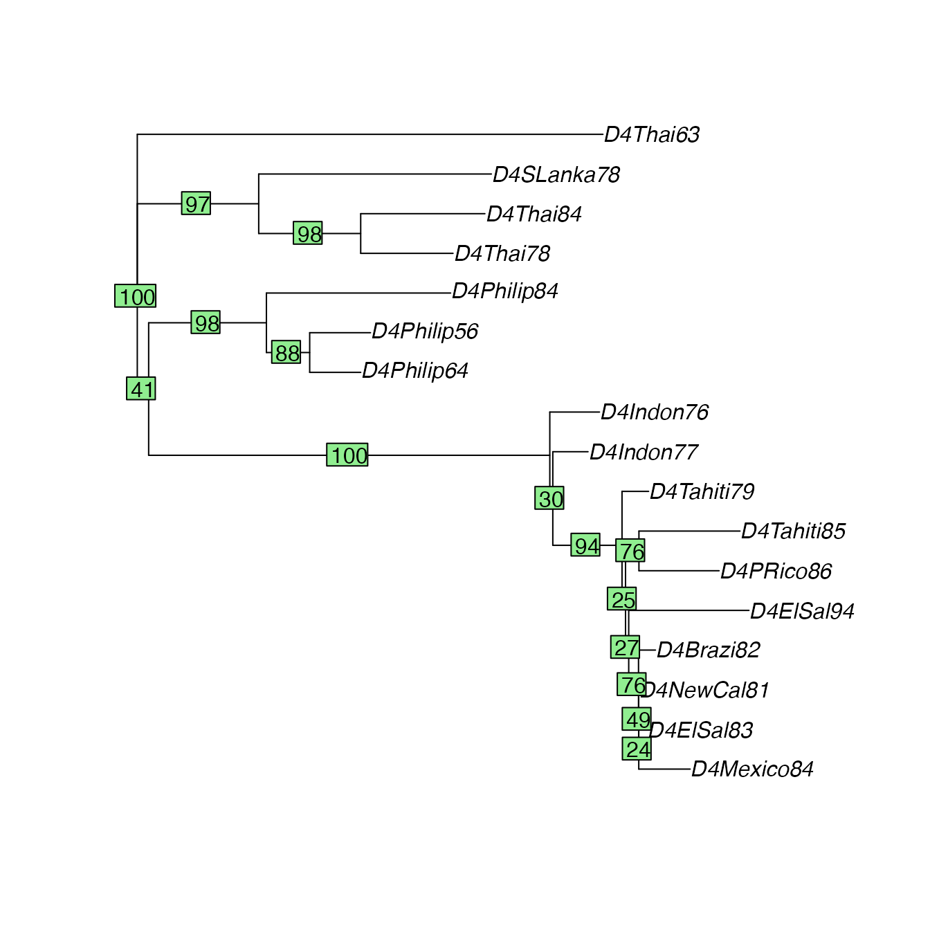

We create a maximum-likelihood (ML) tree and root it as before:

Dfit.ini <- pml(DnjRooted, as.phyDat(DengueSeqs), k=4)
Dfit <- optim.pml(Dfit.ini, optNni=TRUE, optBf=TRUE,
                  optQ=TRUE, optGamma=TRUE, model="GTR")

## Warning: I unrooted the tree

# root:
DfitTreeRooted <- root(Dfit$tree, resolve.root=TRUE, outgroup="D4Thai63")

View the ML tree:

plot(DfitTreeRooted)

Create bootstrap trees:

# bootstrap supports:
DMLboots <- bootstrap.pml(Dfit, optNni=TRUE)
# root:
DMLbootsrooted <- lapply(DMLboots, function(x) root(x, resolve.root=TRUE, outgroup="D4Thai63"))
class(DMLbootsrooted) <- "multiPhylo"

Plot the ML tree again, with bootstrap support values:

plotBS(DfitTreeRooted, DMLboots, type="phylogram")

Using treespace to compare trees

We now use the function treespace to find and plot distances between all these trees:

# collect the trees into a single object of class multiPhylo:
DengueTrees <- c(BEASTtrees, Dnjboots$trees, DMLbootsrooted,
                     DnjRooted, DfitTreeRooted)
class(DengueTrees) <- "multiPhylo"
# add tree names:
names(DengueTrees)[1:200] <- paste0("BEAST",1:200)
names(DengueTrees)[201:300] <- paste0("NJ_boots",1:100)
names(DengueTrees)[301:400] <- paste0("ML_boots",1:100)
names(DengueTrees)[[401]] <- "NJ"
names(DengueTrees)[[402]] <- "ML"
# create vector corresponding to tree inference method:
Dtype <- c(rep("BEAST",200),rep("NJboots",100),rep("MLboots",100),"NJ","ML")

# use treespace to find and project the distances:
Dscape <- treespace(DengueTrees, nf=5)

# simple plot:
plotGrovesD3(Dscape$pco, groups=Dtype)

The function plotGrovesD3 produces interactive d3 plots which enable zooming, moving, tooltip text and legend hovering. We now refine the plot with colour-blind friendly colours (selected using ColorBrewer2), bigger points, varying symbols and point opacity to demonstrate the NJ and ML trees, informative legend title and smaller legend width:

Dcols <- c("#1b9e77","#d95f02","#7570b3")
Dmethod <- c(rep("BEAST",200),rep("NJ",100),rep("ML",100),"NJ","ML")
Dbootstraps <- c(rep("replicates",400),"NJ","ML")
Dhighlight <- c(rep(1,400),2,2)
plotGrovesD3(Dscape$pco, 
             groups=Dmethod, 
             colors=Dcols,
             col_lab="Tree type",
             size_var=Dhighlight,
             size_range = c(100,500),
             size_lab="",
             symbol_var=Dbootstraps,
             symbol_lab="",
             point_opacity=c(rep(0.4,400),1,1), 
             legend_width=80)

We can also add tree labels to the plot. Where these overlap, the user can use “drag and drop” to move them around for better visibility.

plotGrovesD3(Dscape$pco, 
             groups=Dmethod, 
             treeNames = names(DengueTrees), # add the tree names as labels
             colors=Dcols,
             col_lab="Tree type",
             size_var=Dhighlight,
             size_range = c(100,500),
             size_lab="",
             symbol_var=Dbootstraps,
             symbol_lab="",
             point_opacity=c(rep(0.4,400),1,1), 
             legend_width=80)

Alternatively, where labels are too cluttered, it may be preferable not to plot them but to make the tree names available as tooltip text instead:

plotGrovesD3(Dscape$pco, 
             groups=Dmethod, 
             tooltip_text = names(DengueTrees), # add the tree names as tooltip text
             colors=Dcols,
             col_lab="Tree type",
             size_var=Dhighlight,
             size_range = c(100,500),
             size_lab="",
             symbol_var=Dbootstraps,
             symbol_lab="",
             point_opacity=c(rep(0.4,400),1,1), 
             legend_width=80)

The scree plot is available as part of the treespace output:

barplot(Dscape$pco$eig, col="navy")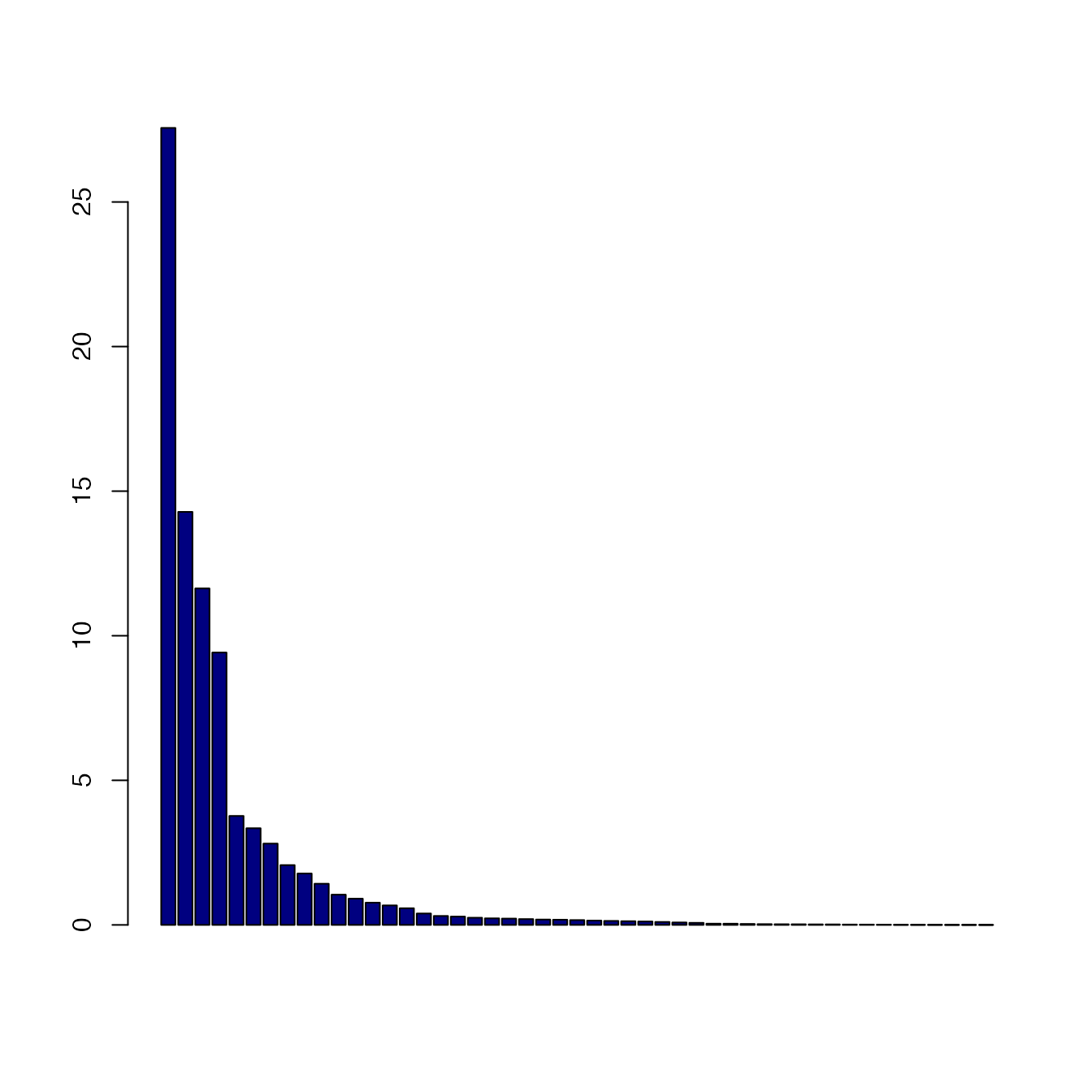

We can also view the plot in 3D:

library(rgl)
Dcols3D <- c(rep(Dcols[[1]],200),rep(Dcols[[2]],100),rep(Dcols[[3]],100),Dcols[[2]],Dcols[[3]])
rgl::plot3d(Dscape$pco$li[,1],Dscape$pco$li[,2],Dscape$pco$li[,3],
       type="s",
       size=c(rep(1.5,400),3,3), 
       col=Dcols3D,
       xlab="", ylab="", zlab="")

treespace analysis

From these plots we can see that treespace has identified variation in the trees according to the Kendall Colijn metric (\(\lambda=0\), ignoring branch lengths). The NJ and ML bootstrap trees have broadly similar topologies but are different from any of the BEAST trees. We can check whether any bootstrap trees have the same topology as either the NJ or ML tree, as follows:

# trees with the same topology as the NJ tree:
which(as.matrix(Dscape$D)["NJ",]==0)

## NJ_boots91         NJ 
##        291        401

# trees with the same topology as the ML tree:
which(as.matrix(Dscape$D)["ML",]==0)

##  ML 
## 402

This shows that the NJ tree has the same topology as one NJ bootstrap tree and one ML bootstrap tree. The ML tree has the same topology as 15 ML bootstrap trees, but no NJ bootstrap trees.

We can compare pairs of trees using the plotTreeDiff function to see exactly where their differences arise. Tips with identical ancestry in the two trees are coloured grey, whereas tips with differing ancestry are coloured peach-red, with the colour darkening according to the number of ancestral differences found at each tip. Since we are comparing the trees topologically (ignoring branch lengths, for the moment), we plot with constant branch lengths for clarity.

# comparing NJ and ML:
plotTreeDiff(DnjRooted,DfitTreeRooted, use.edge.length=FALSE)

treeDist(DnjRooted,DfitTreeRooted)

## [1] 13.93

We can adjust the plot settings to make the visualisation clearer:

# comparing NJ and ML:
plotTreeDiff(DnjRooted,DfitTreeRooted, use.edge.length=FALSE, 
             treesFacing = TRUE, colourMethod = "palette", palette = funky)

For pairwise comparisons it is helpful to find a small number of representative trees. We can find a geometric median tree from the BEAST trees using the medTree function:

BEASTmed <- medTree(BEASTtrees)

There are two median trees, with identical topology:

BEASTmed$trees

## 2 phylogenetic trees

treeDist(BEASTmed$trees[[1]],BEASTmed$trees[[2]])

## [1] 0

so we may select one of them as a BEAST representative tree. Note that for a more thorough analysis it may be appropriate to identify clusters among the BEAST trees and select a summary tree from each cluster: we demonstrate this approach later in the vignette.

BEASTrep <- BEASTmed$trees[[1]]

# comparing BEAST median and NJ:
plotTreeDiff(BEASTrep,DnjRooted, use.edge.length=FALSE, 
             treesFacing = TRUE, colourMethod = "palette", palette = funky)

treeDist(BEASTrep,DnjRooted)

## [1] 13.27

# comparing BEAST median and ML:
plotTreeDiff(BEASTrep,DfitTreeRooted, use.edge.length=FALSE, 
             treesFacing = TRUE, colourMethod = "palette", palette = funky)

treeDist(BEASTrep,DfitTreeRooted)

## [1] 9.487

# comparing BEAST median to a random BEAST tree:
num <- runif(1,1,200)
randomBEASTtree <- BEASTtrees[[num]]
plotTreeDiff(BEASTrep, randomBEASTtree, use.edge.length=FALSE, 
             treesFacing = TRUE, colourMethod = "palette", palette = funky)

treeDist(BEASTrep,randomBEASTtree)

## [1] 5.657

Using treespace to analyse the BEAST trees in more detail:

We used TreeAnnotator (Drummond and Rambaut, 2007) to create a Maximum Clade Credibility (MCC) tree from amongst the BEAST trees.

# load the MCC tree
data(DengueBEASTMCC)
# concatenate with other BEAST trees
BEAST201 <- c(BEASTtrees, DengueBEASTMCC)
# compare using treespace:
BEASTscape <- treespace(BEAST201, nf=5)
# simple plot:
plotGrovesD3(BEASTscape$pco)

There appear to be clusters of tree topologies within the BEAST trees. We can use the function findGroves to identify clusters:

# find clusters or 'groves':
BEASTGroves <- findGroves(BEASTscape, nclust=4, clustering = "single")

and to find a median tree per cluster:

# find median tree(s) per cluster:
BEASTMeds <- medTree(BEAST201, groups=BEASTGroves$groups)
# for each cluster, select a single median tree to represent it:
BEASTMedTrees <- c(BEASTMeds$`1`$trees[[1]],
                   BEASTMeds$`2`$trees[[1]],
                   BEASTMeds$`3`$trees[[1]],
                   BEASTMeds$`4`$trees[[1]])

We can now make the plot again, highlighting the MCC tree and the four median trees:

# extract the numbers from the tree list 'BEASTtrees' which correspond to the median trees: 
BEASTMedTreeNums <-c(which(BEASTGroves$groups==1)[[BEASTMeds$`1`$treenumbers[[1]]]],
                     which(BEASTGroves$groups==2)[[BEASTMeds$`2`$treenumbers[[1]]]],
                     which(BEASTGroves$groups==3)[[BEASTMeds$`3`$treenumbers[[1]]]],
                     which(BEASTGroves$groups==4)[[BEASTMeds$`4`$treenumbers[[1]]]])
# prepare a vector to highlight median and MCC trees
highlightTrees <- rep(1,201)
highlightTrees[[201]] <- 2
highlightTrees[BEASTMedTreeNums] <- 2
# prepare colours:
BEASTcols <- c("#66c2a5","#fc8d62","#8da0cb","#e78ac3")

# plot:
plotGrovesD3(BEASTscape$pco,
          groups=as.vector(BEASTGroves$groups),
          colors=BEASTcols,
          col_lab="Cluster",
          symbol_var = highlightTrees,
          size_range = c(60,600),
          size_var = highlightTrees,
          legend_width=0)

To understand the differences between the representative trees we can use plotTreeDiff again, for example:

# differences between the MCC tree and the median from the largest cluster:
treeDist(DengueBEASTMCC,BEASTMedTrees[[1]])

## [1] 2

plotTreeDiff(DengueBEASTMCC,BEASTMedTrees[[1]], use.edge.length=FALSE, 
             treesFacing = TRUE, colourMethod = "palette", palette = funky)

# differences between the median trees from clusters 1 and 2:
treeDist(BEASTMedTrees[[1]],BEASTMedTrees[[2]])

## [1] 10.63

plotTreeDiff(BEASTMedTrees[[1]],BEASTMedTrees[[2]], use.edge.length=FALSE, 
             treesFacing = TRUE, colourMethod = "palette", palette = funky)

References

[1] Drummond, A. J., and Rambaut, A. (2007) BEAST: Bayesian evolutionary analysis by sampling trees. BMC Evolutionary Biology, 7(1), 214.

[2] Lanciotti, R. S., Gubler, D. J., and Trent, D. W. (1997) Molecular evolution and phylogeny of dengue-4 viruses. Journal of General Virology, 78(9), 2279-2286.